The gap between asymptotic analysis and real execution
Big-O tells you how a cost grows as input grows, in the limit, with constants thrown away. That’s the right tool for comparing two sorting algorithms in a CS class. It’s the wrong tool, on its own, for predicting how a database executes a query. A query planner isn’t picking between abstract algorithms on an idealized machine. It’s picking between concrete physical operations (sequential reads, random reads, hash builds, sort buffers) against a measured data distribution, and it prices them in estimated page fetches and CPU cycles, not big-O classes.
A B-tree lookup is O(log n). A full table scan is O(n). If you stopped there you’d expect the planner to grab the index every time n gets large. Real planners routinely do the opposite, and they’re right to.
Index scan vs. sequential scan
An index scan traverses the B-tree, which is cheap (a handful of comparisons), then for each matching entry fetches the corresponding heap page to get the actual row. That’s a heap fetch, and unless the index is covering, you pay for one per match. Each heap fetch is potentially a random I/O: a different disk page, no locality guarantee, unless the table happens to be physically clustered on that column.
A sequential scan reads the table page by page in physical order. On spinning disks, and even on SSDs behind a page cache, that order benefits from read-ahead and prefetching, which makes it dramatically cheaper per page than scattered random access.
So the comparison isn’t O(log n) vs O(n). It’s closer to this:
index_scan_cost ≈ log(n) [tree traversal]
                 + selectivity * n * random_page_cost  [heap fetches]

seq_scan_cost   ≈ n * seq_page_cost
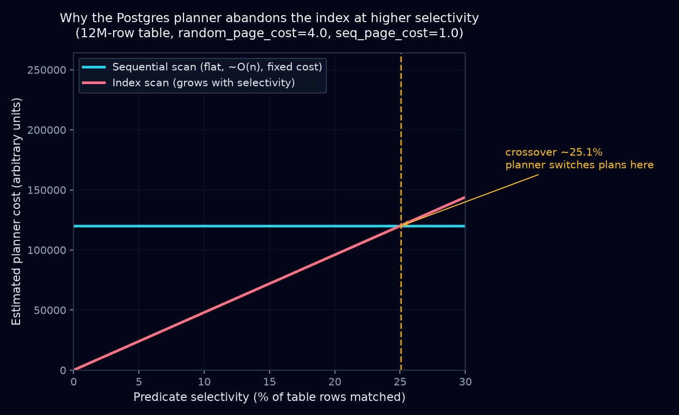
Postgres defaults random_page_cost to 4.0 against a seq_page_cost of 1.0 (people tune it down to around 1.1–1.5 on SSD-backed systems, but it’s still at or above sequential cost). Selectivity is the fraction of rows the predicate is expected to match. Once that fraction gets large enough, the selectivity * n * random_page_cost term outgrows the cost of just reading the whole table in one pass. The crossover usually shows up in the single-digit percentages of the table, not some rare edge case. That’s why an index that’s fantastic for a highly selective predicate turns actively harmful for a low-selectivity one, and the planner refusing to use it is the correct call, not a bug.
The planner doesn’t know Big-O. It knows statistics.
Postgres’s planner is cost-based. It never reasons “index lookup is logarithmic.” It pulls numbers from pg_statistic, populated by ANALYZE: table row count (reltuples), most-common values and their frequencies, histogram bounds for everything else, and correlation between physical row order and column value. From that it computes an estimated selectivity for your predicate, feeds it into the cost formulas above (plus startup cost, CPU tuple cost, CPU operator cost), and picks whichever plan comes out cheapest.
Big-O describes a trend as n approaches infinity. The planner cares about one specific n, one specific selectivity, and specific hardware cost ratios, and it has to estimate all of that. When stats are stale or a predicate correlates with something the optimizer doesn’t model, those estimates can be badly wrong.
An illustrative example (not captured live, representative of real behavior)
Table: orders, 12 million rows, B-tree index on status.
CREATE INDEX idx_orders_status ON orders(status);
ANALYZE orders;
Querying a common status:
EXPLAIN ANALYZE
SELECT * FROM orders WHERE status = 'pending';
Seq Scan on orders (cost=0.00..305412.00 rows=4812000 width=96)
(actual time=0.019..1847.332 rows=4798213 loops=1)
Filter: (status = 'pending'::text)
Rows Removed by Filter: 7201787
Planning Time: 0.112 ms
Execution Time: 1958.410 ms‘pending’ covers roughly 40% of the table. Even with idx_orders_status sitting right there, the planner skips it and does a full scan. That’s correct: fetching 4.8M heap pages randomly through the index would cost far more than one sequential pass, even though the index path is “O(log n) + k” and the seq scan is “O(n).” The constant on the random-access term swamps the asymptotic advantage.
Now a selective status:
EXPLAIN ANALYZE
SELECT * FROM orders WHERE status = 'chargeback_disputed';
Index Scan using idx_orders_status on orders
(cost=0.43..892.17 rows=214 width=96)
(actual time=0.038..0.291 rows=211 loops=1)
Index Cond: (status = 'chargeback_disputed'::text)
Planning Time: 0.098 ms
Execution Time: 0.324 msSelectivity here is about 0.0018%. The heap-fetch term is negligible, and the index wins by roughly four orders of magnitude in wall-clock time, matching the intuitive big-O expectation, because at this selectivity the random-access constant never gets a chance to dominate.
Same table, same index, same schema. Only the data distribution behind the predicate changed, and you can’t see that by studying the index structure on its own.
What to do with this
Indexes aren’t unreliable and seq scans aren’t secretly fast. Complexity class just isn’t enough to predict real execution cost. Four habits follow from that.
Run EXPLAIN (ANALYZE, BUFFERS) before arguing about a plan from intuition. ANALYZE without BUFFERS only shows estimated vs. actual rows and time. BUFFERS shows actual page hits and reads, which is where you’ll catch cases where estimated and actual plans diverge because the stats are stale.
Keep ANALYZE current. Autovacuum handles this most of the time, but bulk loads and fast-churning tables can outrun it, and a bad selectivity estimate produces a bad plan no matter how well you designed the index.
Don’t assume “it has an index, so it’ll use it.” If a predicate commonly matches a large chunk of the table, a partial index (WHERE status != 'pending') or a different approach entirely (a covering index, BRIN for correlated columns, partitioning by status), is usually the real fix. Forcing index usage with planner hints only treats the symptom.
When you’re comparing two query shapes, compare their actual costs on your actual data, not their theoretical complexity class. A nested loop join, asymptotically worse at O(n*m), can still beat a hash join on small, highly selective inner relations, because the hash build’s fixed overhead dominates at small n.
Big-O tells you how a cost scales. The planner has to work out what the cost is for this table, this data and this hardware, and so do you when you’re reading its output. I trust the EXPLAIN output over my asymptotic intuition, because the planner is using a cost function I haven’t memorized and statistics I’ve probably never looked at.